
Introduction
Random numbers(whether true or pseudo) have broad applications for various purposes, including security, monetary transactions, Machine Learning, gaming, statistics, cryptography, simulation, literature, music, and art.
Various tools, machines, and algorithms exist for generating non-colliding random numbers, including the popular Fischer / Knuth Yates algorithm. Besides the popular Fischer / Knuth Yates algorithm, in this article, I’ll show you how you can generate non-colliding pseudo-random numbers using a binary tree with PID (Process IDentifier) without any APIs.
Random Numbers
A sequence of any numbers that cannot be reasonably predicted better than by random chance is generated. This means that the particular outcome sequence will contain some patterns detectable in hindsight but unpredictable to foresight.
Prior to the introduction SecureRandom in Java, the java.util.Random from Oracle JDK 7 implementation makes us of a Linear Congruential Generator method to produce random values in java.util.Random which are easy to predict, and break as an attacker would compute the seed from the output values which take less time than 2^48 attempts, in the case of SecureRandom which provides a cryptographically strong random number that takes random data from the OS that can be an interval between keystrokes and related which are mostly been store in /dev/random and /dev/urandom in case of Linux/Solaris) and uses that as the seed, and produces non-deterministic output.
This article doesn’t focus on true random number generators that generate random numbers, wherein each generation is a function of the current value of a physical environment’s attribute constantly changing in a manner that is practically impossible to model [2]. It rather provides another way of generating non-colliding random numbers(pseudo) using a binary tree with Process ID (PID) similar to the popular Fischer / Knuth Yates algorithm.
Non-Colliding unique random numbers with HashTable
As indicated in the below example, HashTable implementation is the common approach to generating non-colliding random numbers,
Example
Using hashTable to generate a non-colliding and unique random number
Java
HashSet<Integer> storage = new HashSet<>();public void generateRandomValue(){ int currentVal = new SecureRandom(0).next(10); if(!storage.contains(currentVal)){ storage.add(currentVal); } }
The above (just like any other programming language implementation) will work but with many drawbacks including,
1. Memory Usage: It requires additional memory to store the hashed values and maintain the internal data structure. As the dataset grows larger, the memory usage of the HashTable increases accordingly.
2. Hashing Collisions: HashTables are susceptible to collisions based on the defined random size, where different input values produce the same hash value, while some collision handling mechanisms exist, such as separate chaining or open addressing, they, however, introduce complexity and impact performance.
3. Performance Overhead: Inserting and searching for elements in a HashTable involves hash function calculations and potentially traversing collision resolution structures. These operations will introduce additional computational overhead, especially when dealing with a large number of elements. The performance of HashTables would degrade as the dataset size increases.
4. Lack of Sequentiality: HashTables do not provide a built-in mechanism for generating sequential or ordered random numbers. The generated random numbers would appear in a seemingly random order, which might not be suitable for certain applications where sequentiality is desired.
5. Hash Function Selection: The effectiveness of a HashTable relies on the quality of the hash function used. Choosing a suitable hash function that distributes the values evenly and minimizes collisions can be challenging. Inadequate hash functions may result in a higher collision rate and impact the randomness and uniqueness of the generated numbers.
Non-Colliding unique random numbers with BinaryTree PID
Process ID or PID is the process identifier used by most operating system kernels—such as Unix, macOS, and Windows — to identify an active process uniquely. For example, the PID values in Linux, are stored and managed by the operating system kernel in the /proc directory, since each running process is assigned a unique PID by the kernel to identify, this implementation comes with a similar assumption.
Binary Tree PID Approach
Step 0: Start with a dataset of numbers,
Example n = [1, 2, 3, 4, 5, 6, 7, 8, 9, 10,11]
Step 1: Create a binary tree structure with a root node
Step 2: Begin a random cycle (c) to traverse the tree
By default, c = 0, and a cycle is completed when the root, left, and right nodes at each branch have been completely visited.
Step 3: Start at the root node, which is determined by the mid index (n/2) of the dataset.
When c = 0, root_node = n / 2
Step 4:Traverse either the left or right node based on the current cycle:
Left node: c
Right node: (n – 1 ) – c
Step 5: Complete the cycle when the root, left, and right nodes have been visited or check if it’s in the last cycle i.e (c * 3) == (n – 1)
Step 6: Completion check.
If all nodes have been visited (c * 3 == n – 1), increase the next cycle (c) by one, decrease the given index (n) by one, and repeat steps 3 to 6 or check if all nodes are completely visited (i.e n / 2) + 1 == Root(n-1).
Example Walk-through
Example : x = [1, 2, 3, 4, 5, 6, 7, 8, 9, 10]
[1.] Start with cycle (c) = 0
First cycle(c) = 0
Root node = n / 2 (where n is the total number of data)
10 / 2 = 5
X[5] = 6
Left node = c ← 0
X[0] ←1
Right node = (n – c) (When c = 0, assume 1, first traversal)
(10 – 1) ←x[9] ←10
Note: Cycle(0) is completed (i.e all nodes at that cycle have been completely visited)
generated random numbers with zero collision ⇐ [6, 1, 10] (root, left, right)
[1, 10, 6] (left, right, root)
[10, 1, 6] (right, left, root)
[2.] Check if it has reached the last cycle ⇐ (c * 3) == (n – 1) or (n / 2) + 1 == (n – 1) ?
(0 * 3) != (10 – 1)
(10 / 2) + 1 != (10 – 1)
[3.] Increase the next cycle(c) by one(1), c ←1
Decrease the given index(n) by one, n ←9
Second cycle(c) = 1
Root node = n / 2 (where n is the total number of data)
9 / 2 = 4
X[4] = 5
Left node = c ← 1
X[1] ←2
Right node = (n – c )
(9 – 1) ←x[8] ←9
Cycle(1) is completed (i.e root, left, and right already visited) node has been visited
generated_random_numbers ⇐ [6, 1, 10, 5, 2, 9] (root, left, right, root, left, right)
[1, 10, 6, 2, 5, 9] (left, right, root, left, root, right)
[10, 1, 6, 9, 2, 5] (right, left, root, right, left, root)
[2.] Check if it has reached the last cycle ⇐ (c * 3) == (n – 1) or (n / 2) + 1 == (n – 1)?
(1 * 3) != (9 – 1)
(9 / 2) + 1 != (9 – 1)
[3.] Increase the next cycle(c) by one(1), c ←2
Decrease the given index(n) by one, n ←8
Third cycle(c) = 2
Root node = 8 / 2 (where n is the total number of data)
9 / 2 = 4
X[4] = 5
Left node = c ← 1
X[1] ←2
Right node = (n – c )
(9 – 1) ←x[8] ←9
Cycle(2) is completed (i.e root, left, and right already visited) node has been visited
generated_random_numbers ⇐ [6, 1, 10, 5, 2, 9] (root, left, right, root, left, right)
[1, 10, 6, 2, 5, 9] (left, right, root, left, root, right)
[10, 1, 6, 9, 2, 5] (right, left, root, right, left, root)
Cycle Table
| Cycle {c} 0 | 1 | 2 | ||
| Node(n = 10) | n=10 | n=9 | n=8 | |
| Root (n / 2) | n/2 = 5; x[5] == 6 | x[9/2] == 5 | x[8/2] == 4 | |
| Left { c } | X[0] == 1 | X[1] == 2 | X[2] == 3 | |
| Right (n – 1) – c | (10 – 1); x[9] == 10 | X[ (9-1 ] == 9 | X[8-1] == 8 | x[(n-1-1)] X[8-1-1]] = 7 |
| Unique random numbers | 6,1,10 or 10, 6, 1 | 10,1,6,2,9,5 or 10, 6, 1, 5, 9, 2 | 10, 6, 1, 5, 9, 2,8, 4,3 | …. |
Many predictable, and unpredictable unique, and non-colliding random number patterns can be generated from the above as
[1.] 6, 1, 10, 5, 2, 9, 4, 3, 8, 7
[2.] 10, 1, 6, 2, 5, 9, 3, 8, 7, 4
[3.] 7, 1, 6, 10, 2, 5, 9, 3, 4, 8
[4.] 8, 4, 3, 2, 5, 9, 7, 1, 6, 10
[5.] 7, 4, 8, 3, 2, 9, 5, 10, 1, 6
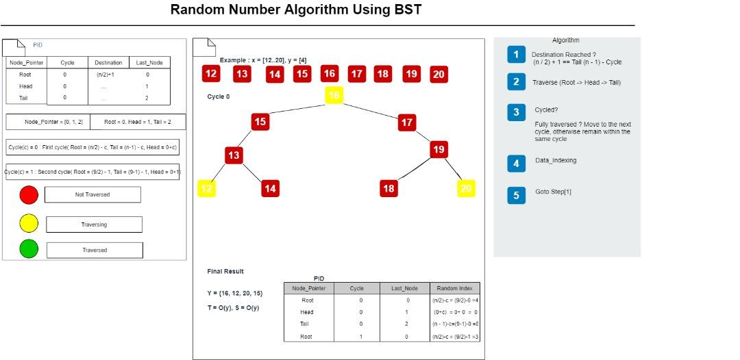
Fig.1 (Random Number Algorithm using B-Tree, Author’s own figure)
The above implementation of a Binary Tree with PID for generating non-colliding random numbers offers several advantages and can be beneficial in various use cases:
Advantages
1. Non-Colliding Random Numbers: The foremost advantage is the generation of non-colliding random numbers. By leveraging the tree structure and process identifiers (PIDs), the implementation ensures that duplicates are eliminated, providing unique random numbers.
2. Deterministic and Reproducible: The deterministic nature of the algorithm ensures that the same dataset and starting conditions will always produce the same random number sequence. This reproducibility can be valuable in scenarios where consistent random numbers are required for testing, debugging, or result validation.
3. Efficient Memory Usage: The Binary Tree with PID implementation is memory-efficient compared to other approaches like HashTables.
4. Sequentiality and Order: The algorithm generates random numbers in a sequential manner based on the tree traversal. This sequentiality maintains an unknown defined order specified by the user, which can be advantageous in applications where ordered random numbers are desired, such as simulations or iterative algorithms.
Use cases
1. Gaming: Generating unique random numbers is crucial in games to ensure fair gameplay, random events, and unique outcomes.
2. Simulations: Simulations often require a large number of random inputs, and ensuring non-colliding random numbers would enhance the accuracy and reliability of the simulation results.
3. Cryptography: Random numbers play a vital role in cryptographic algorithms. The non-colliding nature of the generated random numbers can also strengthen cryptographic security.
4. Testing and Debugging: The deterministic and reproducible nature of the algorithm makes it valuable for testing and debugging purposes, where consistent random inputs are needed to reproduce specific scenarios.
Disadvantages
1. Dependency on PIDs: The reliance on process identifiers (PIDs) assumes the availability and uniqueness of PIDs within the operating system. This dependency might limit the algorithm’s applicability in certain environments or scenarios where PIDs are not readily accessible.
2. Collision Handling for PID Reuse: If PIDs are recycled or reused by the operating system, collision handling mechanisms might be required to handle cases where the same PID is encountered again.
3. Parallel Execution: The current implementation does not address parallel execution or concurrency for random numbers.
4. Optimal Tree Structure: Depending on the dataset characteristics, different tree structures (e.g., balanced binary trees) might be explored to improve performance and reduce traversal times.
The need for true and untrue random numbers depends on your goal.

Leave a comment